Assisting the Adversary to Improve GAN Training
Andreas Munk, William Harvey & Frank Wood
IJCNN 2021
amunk@cs.ubc.ca
March 26, 2021
Table of Contents
- Closing the gap between theory and practice
- Generative adversarial networks (GANs) cite:goodfellow2014generative
- Why GANs?
- The optimal adversary assumption and the minimization of divergences
- Does an optimal adversary lead to optimal gradients?
- Adversary constructors
- Assisting the Adversary - introducing AdvAs
- Removing the hyperparameter \(\lambda\)
- Experiments
- MNIST and WGAN-GP cite:gulrajani2017improved
- CelebA and StyleGan cite:karras2020analyzing
- References
Closing the gap between theory and practice
- The GAN framework is a minimax game, that pivots an adversary (critic/discriminator) against a generator
- The adversary is often assumed optimal in theoretical analysis and in the
construction of different GANs
- In practice this is essentially never true
- We consider a largely overlooked approach to constraining GAN training
mescheder2017numerics,nagarajan2017gradient
- Re-motivated to bridge the gap between theory and practice
- Accounts for the adversary being suboptimal - The Adversarys Assistant
(AdvAs) munk2020assisting
- A regularizer which encourages the generator to move towards points where the current adversary is optimal
Generative adversarial networks (GANs) goodfellow2014generative
- A generator is a neural network \(g:\gZ\rightarrow\gX\subseteq\real^{D_{x}}\)
which maps from a random vector \(\vz\in\gZ\) to an output \(\vx \in \gX\)
- \(g\) characterizes a distribution \(p_{\theta}(\vx)\), where \(\theta\in\Theta\subseteq\mathbb{R}^{D_g}\) denotes the generator’s parameters
- Aim is to match \(p_{\theta}\) with some real target distribution \(p_{\mr{true}}\)
- An adversary \(a_\phi:\gX\rightarrow \gA\) with parameters \(\phi\in\Phi\subseteq\real^{D_a}\)
Generally we frame GANs as a minimax game,
\[\min_{\theta}\max_{\phi}h(p_{\theta},a_\phi)\]
- If the minimax game of perfectly solved, then \(p_{\theta} = p_{\mr{true}}\)
Originally Goodfellow et al. (2014) defined \(\gA=\br{0,1}\)
\[ h(p_{\theta},a_\phi) = \mathbb{E}_{x\sim p_{\mr{true}}} \left[ \log a_\phi(x) \right] + \mathbb{E}_{x\sim p_{\theta}} \left[ \log (1- a_\phi(x)) \right].\]
Why GANs?
- Generative modeling using implicit densities
- Produce photo-realistic images zhou2019hype
- However, they tend to have unstable training dynamics mescheder2018which
- Primarily addressed using different GAN objectives or by using various regularization techniques when training the adversary
- We focus on regularizing the training of the generator
- Compatible with above-mentioned regularization techniques
The optimal adversary assumption and the minimization of divergences
- Before each generator update, the adversary is assumed optimal
- That is, if \(\gF\) is the class of permissible adversary functions, then for a particular \(\theta\) the adversary is optimal if \(a^{*}=\argmax_{a \in \gF}h(p_{\theta},a)\)
When \(a\) is parameterized by a neural net with parameters \(\phi\in\Phi\), we define
\[\Phi^*(\theta) = \{\phi \in \Phi \mid h(p_\theta, a_\phi) = \max_{a \in \gF}h(p_{\theta},a) \}\]
This assumption turns the two-player minimax game into a case of minimizing an objective w.r.t. \(\theta\) alone
\[ \gM(p_{\theta}) = \max_{a \in \gF}h(p_{\theta},a) = h(p_\theta, a_{\phi^*}) \quad \text{where} \quad \phi^*\in\Phi^*(\theta). \]
- For instance goodfellow2014generative showed that \(\gM(p_{\theta}) = 2\cdot\text{JSD}(p_{\mr{true}} || p_\theta) - \log 4\)
- Many other GAN approaches make use of the optimal adversary assumption to show that \(\gM(p_{\theta})\) reduces to some divergence (e.g. WGAN arjovsky2017wasserstein)
Does an optimal adversary lead to optimal gradients?
- The goal of training the generator can be seen as minimizing \(\gM(p_{\theta})\)
- In practice the generator update requires it’s gradient \(\grad_\theta \gM(p_{\theta})\) (e.g. gradient descent)
- Assume we have generator parameters \(\theta'\). Consider
\(\phi^*\in\Phi^*(\theta')\) such that \(h (p_{\theta'}, a_{\phi^*})\) and
\(\gM(p_{\theta'})\) are equal in value
- We want \(\grad_\theta \gM(p_{\theta})\mid_{\theta=\theta'}\) but calculate in
practice the partial derivative \(D_1 h (p_\theta,
a_{\phi^*})\mid_{\theta=\theta'}\)
- Where we defined \(D_1 h (p_\theta, a_\phi)\) to denote the partial derivative of \(h(p_\theta, a_\phi)\) with respect to \(\theta\) with \(\phi\) kept constant. Similarly, define \(D_2 h (p_\theta, a_\phi)\) to denote the derivative of \(h (p_\theta, a_\phi)\) with respect to \(\phi\), with \(\theta\) held constant.
- It is not immediately obvious these two quantities are equal
- We want \(\grad_\theta \gM(p_{\theta})\mid_{\theta=\theta'}\) but calculate in
practice the partial derivative \(D_1 h (p_\theta,
a_{\phi^*})\mid_{\theta=\theta'}\)
- By extending Theorem 1 in milgrom2002envelope we have that
Theorem 1. Let \(\gM(p_{\theta})=h(p_{\theta},a_{\phi^*})\) for any \(\phi^*\in\Phi^{*}(\theta)\). Assuming that \(\gM(p_{\theta})\) is differentiable w.r.t. \(\theta\) and \(h(p_{\theta},a_{\phi})\) is differentiable w.r.t. \(\theta\) for all \(\phi\in\Phi^{*}(\theta)\), then if \(\phi^{*}\in\Phi^{*}(\theta)\) we have \[ \grad_{\theta}\gM(p_{\theta})=D_1 h(p_{\theta},a_{\phi^{*}}) \]
Adversary constructors
An adversary constructor is a function \(f:\Theta\rightarrow\Phi\), where for all \(\theta \in \Theta\), \(f(\theta) = \phi^*\in\Phi^{*}(\theta)\),
\[h(p_{\theta},a_{f(\theta)})=\max_{a\in\gF}h(p_{\theta},a)\]
We cannot compute the function \(f(\theta)\) in general. However, they lead to a condition which must be satisfied for Theorem 1 to be invoked
Corollary 1. Let \(f:\Theta\rightarrow\Phi\) be a differentiable mapping such that for all \(\theta \in \Theta\), \(\gM(p_{\theta})=h(p_{\theta},a_{f(\theta)})\). If the conditions in Theorem 1 are satisfied and the Jacobian matrix of \(f\) with respect to \(\theta\), \(\mJ_{\theta}(f)\) exists for all \(\theta\in\Theta\) then
\begin{equation}\label{eq:cor} \trans{D_2 h(p_{\theta},a_{f(\theta)})} \mJ_{\theta}(f) = 0. \end{equation}
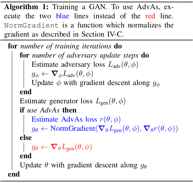
Assisting the Adversary - introducing AdvAs
- Eq. \ref{eq:cor} is a necessary condition for invoking Theorem 1
- \(\trans{D_2 h(p_{\theta},a_{f(\theta)})} \mJ_{\theta}(f)\) could be viewed as a
measure of “closeness”.
- Cannot be computed
- Can compute \(D_2 h(p_{\theta},a_{\phi})\)
- Use the magnitude as an approximate measure of how “close” we are to having an optimal adversary
Define the objective functions
\begin{align} \grad_\theta L_{\text{gen}}(\theta, \phi) &= \grad_\theta h(p_{\theta},a_\phi) \nonumber \\ \grad_\phi L_{\text{adv}}(\theta, \phi) &= -\grad_\phi h(p_{\theta},a_\phi) \nonumber \end{align}Using AdvAs implies
\[ L^{\mr{AdvAs}}_{\mr{gen}}(\theta,\phi) = L_{\mr{gen}}(\theta,\phi) + \lambda\cdot r(\theta,\phi) \]
with \(r(\theta,\phi) = \norm{\grad_\phi {L_{\mr{adv}}}(\theta,\phi)}_2^2\) and \(\lambda\) being a hyperparameter.
- Preserves convergence results:
- Using AdvAs does not interfere with adversary updates
- Assuming an optimal adversary we have \(L^{\mr{AdvAs}}_{\mr{gen}}(\theta,\phi) \rightarrow L_{\text{gen}}(\theta, \phi)\)
- Use an unbiased estimate \(\tilde{r}(\theta, \phi) \approx \norm{\grad_\phi
{L_{\mr{adv}}}(\theta,\phi)}_2^2\)
- consider two independent and unbiased estimates of \(\grad_\phi {L_{\mr{adv}}}(\theta,\phi)\) denoted \(\mX,\mX'\). Then \(\E\br{\trans{\mX}\mX'}=\trans{\E\br{\mX}}\E\br{\mX'}=\norm{\grad_{\phi}L_{\mr{adv}}(\theta,\phi)}_2^2\).
Removing the hyperparameter \(\lambda\)
- If \(\lambda\) is too large it may destabilize training. If too small it is equivalent to not using AdvAs.
Define
\begin{align*} \vg_{\mr{orig}}(\theta, \phi) &= \grad_{\theta}L_{\mr{gen}}(\theta,\phi) \\ \vg_{\mr{AdvAs}}(\theta, \phi) &= \grad_{\theta}\tilde{r}(\theta,\phi) \\ \vg_{\mr{total}}(\theta, \phi, \lambda) &= \grad_{\theta}L^{\mr{AdvAs}}_{\mr{gen}}(\theta,\phi) \\ &= \vg_{\mr{orig}}(\theta, \phi) + \lambda \vg_{\mr{AdvAs}}(\theta, \phi). \end{align*}- We set
Experiments
MNIST and WGAN-GP gulrajani2017improved
- The best FID score reached is improved by \(28\%\) when using AdvAs

Figure 1: FID scores throughout training for the WGAN-GP objective on MNIST, estimated using 60,000 samples from the generator. We plot up to a maximum of 40,000 iterations. When plotting against time (right), this means some lines end before the two hours we show. The blue line shows the results with AdvAs, while the others are baselines with different values of \(n_{\mr{adv}}\), the number of adversary updates per generator update.
CelebA and StyleGan karras2020analyzing

Figure 2: Bottom: FID scores throughout training estimated with \(1000\) samples, plotted against number of epochs (left) and training time (right). FID scores for AdvAs decrease more on each iteration at the start of training and converge to be \(7.5\%\) lower. Top: The left two columns show uncurated samples with and without AdvAs after 2 epochs. The rightmost two columns show uncurated samples from networks at the end of training. In each grid of images, each row is generated by a network with a different training seed and shows 3 images generated by passing a different random vector through this network. AdvAs leads to obvious qualitative improvement early in training.