Generative Modeling by Estimating Gradients of the Data Distribution
By Yang Song† & Stefano Ermon†
†Stanford University
Presented By
Andreas Munk
amunk@cs.ubc.ca
May 12, 2020
Table of Contents
- Generative Modeling by Estimating Gradients of the Data Distribution cite:song2019generative
- Langevin Dynamics cite:wibisono2018sampling
- Score Matching cite:hyvarinen2005estimation
- Sliced Score Matching cite:song2019sliced
- Denoising Score Matching cite:vincent2011connection
- Langevin Dynamics in the Noise Perturbed Manifold
- Why?
- Annealed Langevin Dynamics
- Practical Considerations
- Experiments
- Conclusion
- References
Generative Modeling by Estimating Gradients of the Data Distribution song2019generative
- Likelihood-free generative modeling
- Propose an annealed Langevin Dynamics
- Based on score matching
- Main benefits:
- No adversarial methods
- Does not require sampling from the model during training
- Provides for a principled way for model comparison (within the same framework)
- Achieve state-of-the-art inception score on CIFAR-10
Langevin Dynamics wibisono2018sampling
- \(X\) is a random variable in \(\real^{d}\)
- \(p\) is a differentiable target density
- \(W\) is the standard Brownian motion (in \(\real^{d}\))
- Langevin Dynamics are: \[\dm{X}_{t} = \grad \ln p(X_t)\dm{t} + \sqrt{2}\dm{W}_{t}\] with the distribution of \(X_{t}\) following these dynamics converging to \(p\)
- The discretized version for small time steps \(\epsilon\) is \[\Delta \vx = \grad_{\vx}\ln p(\vx)\epsilon + \vz,\quad \vz\sim\mN(0,\sqrt{2\epsilon}\mI)\]
- Equivalently \[\vx_{t+1}\sim\mN(\vx_{t}+\grad_{\vx}\ln p(\vx)\epsilon, \sqrt{2\epsilon}\mI)\]
- May correct for the discretization error using Metropolis-Hastings with proposal \[q(\vx_{t+1}|\vx_{t}) =\mN(\vx_{t}+\grad_{\vx}\ln p(\vx)\epsilon, \sqrt{2\epsilon}\mI)\]
- Assuming \(\epsilon\) is small enough and t is sufficiently large, the acceptance rate goes to one
- Used also for inference - see e.g. Stochastic Gradient Langevin Dynamics welling2011bayesian
- Think of Langevin Dynamics as a form of a Markov Chain
Score Matching hyvarinen2005estimation
- Can we estimate \(\grad_{\vx}\ln p(\vx)\)?
- Define \(s_{\theta}(\vx)=\grad_{\vx}\ln q_{\theta}(\vx), ~s_{\theta}:\real^{d}\rightarrow\real^{d}\)
- Train \(s_{\theta}\) to match \(\grad_{\vx}\ln p(\vx)\) by minimizing, \[\begin{align*}J(\theta)&=\frac{1}{2}\E_{p(\vx)}\br{\norm{s_{\theta}(\vx) - \grad_{\vx}\ln p(\vx)}^2} \\ &= \E_{p(\vx)}\br{\mr{tr}(\grad_{\vx}s_{\theta}(\vx)) + \frac{1}{2}\norm{s_{\theta}(\vx)}^2} + \mr{const}\end{align*}\]
- Consistency: Assuming \(\exists\theta^{*}(s_{\theta^{*}}(\vx)=\grad_{\vx}\ln p(\vx))\) then \(J(\theta)=0\Leftrightarrow\theta=\theta^{*}\)
- Involves Jacobian of (Hessian of \(q\))
- Weak regularity conditions:
- \(p(\vx)\) is differentiable
- \(\E_{p(\vx)}\br{\norm{s_{\theta}(\vx)}^{2}}<\infty,~\forall \theta\)
- \(\E_{p(\vx)}\br{\norm{\grad_{\vx}\ln p(\vx)}^{2}}<\infty\)
- \(\lim\limits_{\norm{\vx}\rightarrow\infty} p(\vx)s_{\theta}(\vx)=\vec{0},~\forall \theta\)
Proofs of the Objective Reduction
- We need only consider \(-\intd{\vx}p(\vx)\trans{s_{\theta}(\vx)}\grad_{\vx}\ln p(\vx)=-\sum_{i}\intd{\vx}p(\vx)s_{i}(\vx)\frac{\pp \ln p(\vx)}{\pp x_{i}}=-\sum_{i}\intd{\vx}s_{i}(\vx)\frac{\pp p(\vx)}{\pp x_{i}}\), where \(s_{i}(\vx)=s_{\theta}(\vx)_{i}\)
- We restrict our attention to a single \(i\) as the derivation holds for every \(i\)
- Using the shorthand notation \(\pp_{i}f(\vx)=\frac{\pp f(\vx)}{\pp x_{i}}\) we now prove that \[\intd{\vx}s_{i}(\vx)\pp_{i}p(\vx)=-\intd{\vx}p(\vx)\pp_{i}s_{i}(\vx)\]
- Recall that for a differentiable function \(h(\vx)=p(\vx)s_{i}(\vx)\) we have \[\pp_{i}h(\vx)=\pp_{i}\paren{p(\vx)s_{i}(\vx)} = p(\vx)\pp_{i}s_{i}(\vx)+s_{i}(\vx)\pp_{i}p(\vx)\] and so \[\int_{b}^{a}\dm{x_{i}}\pp_{i}h(\vx) = h(x_{1},\dots,x_{i-1},a,x_{i+1},\dots,x_{d}) -h(x_{1},\dots,x_{i-1},b,x_{i+1},\dots,x_{d}) = \int_{b}^{a}p(\vx)\pp_{i}s_{i}(\vx)+s_{i}(\vx)\pp_{i}p(\vx)\dm{x_{i}}\]
- From the regularity conditions we have \(\lim\limits_{\norm{\vx}\rightarrow\infty} p(\vx)s_{\theta}(\vx)=\vec{0},~\forall \theta\), \[\int_{-\infty}^{\infty}\dm{x_{i}}\pp_{i}h(\vx) = \lim\limits_{a\rightarrow\infty,b\rightarrow-\infty} \br{h(x_{1},\dots,x_{i-1},a,x_{i+1},\dots,x_{d}) -h(x_{1},\dots,x_{i-1},b,x_{i+1},\dots,x_{d})}=0\] \[\Downarrow\] \[\int_{-\infty}^{\infty}p(\vx)\pp_{i}s_{i}(\vx)\dm{x_{i}} = -\int_{-\infty}^{\infty}s_{i}(\vx)\pp_{i}p(\vx)\dm{x_{i}}\]
- Additional outer integrals does not change this and so we have \[\intd{\vx}s_{i}(\vx)\pp_{i}p(\vx)=-\intd{\vx}p(\vx)\pp_{i}s_{i}(\vx) = -\E_{p(\vx)}\br{\pp_{i}s_{i}(\vx)}\]
- Identifying \[\sum_{i=1}^{d}\pp_{i}s_{i}(\vx) = \mr{tr}(\grad_{\vx}s_{\theta}(\vx))\] concludes the proof
Sliced Score Matching song2019sliced
- Preferably no Jacobian in score matching
- Projects the score functions onto a random direction \(\vv\in\real^{d}\)
- Leads to the following objective
\[\begin{align*}J_{\mr{SSM}}(\theta)
&=\frac{1}{2}\E_{p(\vv)}\br{\E_{p(\vx)}\br{\norm{\trans{\vv} s_{\theta}(\vx) -
\trans{\vv}\grad_{\vx}\ln p(\vx)}^2}}
\\ &=\E_{p(\vv)}\br{\E_{p(\vx)}\br{\trans{\vv}\grad_{\vx}s_{\theta}(\vx)\vv +
\frac{1}{2}(\trans{\vv} s_{\theta}(\vx))^{2}}} + \mr{const}\end{align*}\]
- If \(p(\vv)=\mN(0,\mI)\), \[\E_{p(\vv)}\br{(\trans{\vv} s_{\theta}(\vx))^{2}} =\norm{s_{\theta}(\vx)}^{2}\]
- Similar weak regularity conditions and satisfies consistency
Algorithmic Differences
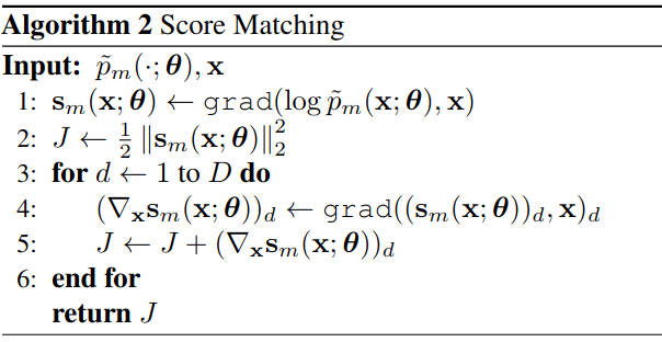
Figure 1: Score matching algorithm
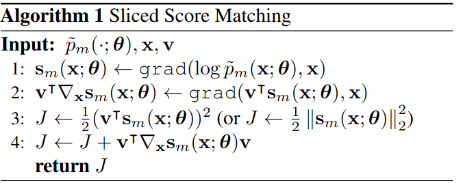
Figure 2: Sliced score matching algorithm
Denoising Score Matching vincent2011connection
- Induce noise pertubation of the data via some “pertubation” distribution
- \(\sigma\) denotes noise level
- Objective: \[\begin{align*}J_{\mr{NSM}}(\theta) &=\frac{1}{2}\E_{p_{\sigma}(\tilde{\vx}|\vx)p(\vx)}\br{ \norm{s_{\theta}(\tilde{\vx}) - \grad_{\tilde{\vx}}\ln p_{\sigma}(\tilde{\vx}|\vx)}^2} \\ &=\E_{p_{\sigma}(\tilde{\vx}|\vx)p(\vx)}\br{ \frac{1}{2}\norm{s_{\theta}(\tilde{\vx})}^{2} - \trans{s_{\theta}(\tilde{\vx})}\grad_{\tilde{\vx}}\ln p_{\sigma}(\tilde{\vx}|\vx)} + \mr{const}\end{align*}\]
- No Jacobian term
- Minimizing \(J_{\mr{NSM}}\) is equivalent to solving for the optimal \(\theta^{*}\) such that \[s_{\theta^{*}}(\tilde{\vx}) = \grad_{\tilde{\vx}}\ln\intd{\vx p(\vx)} p_{\sigma}(\tilde{\vx}|\vx) =\grad_{\tilde{\vx}}\ln p_{\sigma}(\tilde{\vx})\]
- Notice that as \(\sigma\rightarrow 0\) then
\(p_{\sigma}(\tilde{\vx})\rightarrow p(\vx)\)
- Exploited by song2019generative
Proofs of the Minimization Equivalence
- We prove that minimizing \(J_{\mr{NSM}}(\theta)\) is equivalent to minimizing \[J_{\mr{D}}(\theta)=\frac{1}{2}\E_{p_{\sigma}(\tilde{\vx})}\br{ \norm{s_{\theta}(\tilde{\vx}) - \grad_{\tilde{\vx}}\ln p_{\sigma}(\tilde{\vx})}^2}\]
- We need only show that \[\begin{equation}\label{eq:to-prove}\E_{p_{\sigma}(\tilde{\vx})}\br{ \trans{s_{\theta}(\tilde{\vx})}\grad_{\tilde{\vx}}\ln p_{\sigma}(\tilde{\vx})} = \E_{p_{\sigma}(\tilde{\vx}|\vx)p(\vx)}\br{ \trans{s_{\theta}(\tilde{\vx})}\grad_{\tilde{\vx}}\ln p_{\sigma}(\tilde{\vx}|\vx)}\end{equation}\]
- Notice that \[\begin{equation}\label{eq:grad-marg}\grad_{{\tilde{\vx}}}\ln p_{\sigma}(\tilde{\vx}) = \grad_{\tilde{\vx}}\ln\intd{\vx}p_{\sigma}(\tilde{\vx}|\vx)p(\vx) = \frac{1}{p_{\sigma}(\tilde{\vx})} \intd{\vx}\grad_{\tilde{\vx}}p_{\sigma}(\tilde{\vx}|\vx)p(\vx) \end{equation}\]
- Substituting \ref{eq:grad-marg} into the expression of the left-hand side of \ref{eq:to-prove} we find \[\begin{align*}\E_{p_{\sigma}(\tilde{\vx})}\br{ \trans{s_{\theta}(\tilde{\vx})}\grad_{\tilde{\vx}}\ln p_{\sigma}(\tilde{\vx})} &= \int\trans{s_{\theta}(\tilde{\vx})} \int\grad_{\tilde{\vx}}p_{\sigma}(\tilde{\vx}|\vx)p(\vx) \dm{\vx}\dm{\tilde{\vx}} \\ &= \int\int \trans{s_{\theta}(\tilde{\vx})}\grad_{\tilde{\vx}}\ln p_{\sigma}(\tilde{\vx}|\vx)p_{\sigma}(\tilde{\vx}|\vx)p(\vx) \dm{\vx}\dm{\tilde{\vx}} \\ &= \E_{p_{\sigma}(\tilde{\vx}|\vx)p(\vx)}\br{ \trans{s_{\theta}(\tilde{\vx})}\grad_{\tilde{\vx}}\ln p_{\sigma}(\tilde{\vx}|\vx)}\end{align*}\]
- Leading to \[J_{\mr{DSM}}(\theta)=J_{\mr{D}}(\theta) + C,\] where \(C\) is a constant equal to the difference between the constant terms of \(J_{\mr{NSM}}(\theta)\) and \(J_{\mr{D}}(\theta)\)
Langevin Dynamics in the Noise Perturbed Manifold
- Perturb data with Gaussian noise - \(\mN(0,\sigma)\)
- Train noise conditional score estimator
\(s_{\theta}(\tilde{\vx},\sigma)\approx\grad_{\tilde{\vx}}\ln
p_{\sigma}(\tilde{\vx})\) (Deep Neural Network)
- Called Noise Conditional Score Network (NCSN)
- Employ Langevin Dynamics in the perturbed space using
\(s_{\theta}(\tilde{\vx},\sigma)\)
- Ensured to be in \(\real^{d}\)
Why?
- The denoising score matching objective has no Jacobian terms
- The theory behind score matching requires a well-defined \(p(\vx)\) everywhere
in \(\real^{d}\)
- Typically \(p(\vx)\) has a support restricted to some low dimensional manifold embedding in the ambient space
- Langevin dynamics (LD) is likely to mix poorly if \(p(\vx)\) has large regions
with near-zero probability
- May additionally lead to poor training of \(s_{\theta}(\vx)\)
\(p(\vx)=\frac{1}{5}\mN((-5,-5),\mI) + \frac{4}{5}\mN((5,5),\mI)\)
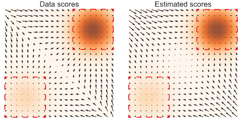
Figure 3: Left \(\grad_{\vx}\ln p(\vx)\). Right \(s_{\theta}(\vx)\). Darker color implies higher density. Squares are regions where \(s_{\theta}(\vx)\approx\grad_{\vx}\ln p(\vx)\)
\(p(\vx)=\frac{1}{5}\mN((-5,-5),\mI) + \frac{4}{5}\mN((5,5),\mI)\)
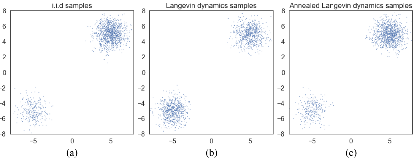
Figure 4: Samples from \(p(\vx)\) using different methods. a) Exact sampling b) Using LD with exact score c) Annealed LD
Annealed Langevin Dynamics
- Intuition:
- Large noise level forms “bridges” across regions with low probability
- Improves mixing of the Langevin dynamics
- Anneal noise level to converge to “true” data distribution
- Define noise levels as a geometric sequence \(\tub{\sigma_{i}}_{i=1}^{L}\)
- \(\frac{\sigma_{1}}{\sigma_{2}}=\dots=\frac{\sigma_{L-1}}{\sigma_{L}}>1\)
- Train noise conditional score estimator \(s_{\theta}(\tilde{\vx},\sigma_{i})\) for every
level
- noise distribution \(p_\sigma(\tilde{\vx}|\vx)=\mN(\vx,\sigma^{2}\mI)\)
- noise level objective \[l(\theta,\sigma)\triangleq J_{\mr{DSM}(\theta,\sigma)}= \frac{1}{2}\E_{p_{\sigma}(\tilde{\vx}|\vx)p(\vx)}\br{ \norm{s_{\theta}(\tilde{\vx},\sigma) + \frac{\tilde{\vx}-\vx}{\sigma^{2}}}^{2}}\]
- unified objective using an objective “weight” \(\lambda(\sigma)>0\) \[\mL\paren{\theta,\tub{\sigma_{i}}_{i=1}^{L}}\triangleq \frac{1}{L}\sum_{i=1}^{L}\lambda(\sigma_{i})l(\theta,\sigma_{i})\]
- set \(\lambda(\sigma)=\sigma\)
- empirically showed \(\lambda(\sigma)l(\theta,\sigma)\) to be independent of \(\sigma\)
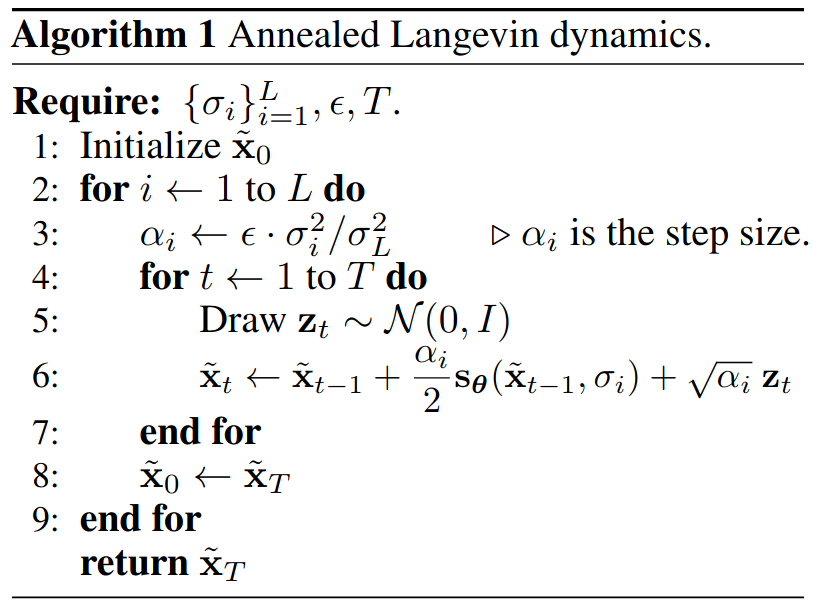
- The final sample of each noise level LD process initializes the next process
- Additionally \(s_{\theta}(\tilde{\vx})\) is likely well estimated in the traversed regions at the different noise levels
- Samples from \(q_{\theta}(\vx)\) by running several “MCMC-like” chains
Practical Considerations
- Step size \(\alpha_{i}\)
- Should decrease over time to ensure convergence welling2011bayesian
- Held fixed at each noise level for NCSNs
- Number of steps \(T\)
- Noise levels \(\tub{\sigma_{i}}_{i=1}^{L}\)
Experiments
Experimental Setup
- \(\tub{\sigma_{i}}_{i=1}^{10}=\tub{1,\dots,0.01}\)
- \(T=100,~\epsilon=2\times10^{-5}\)
MNIST, CelebA and CIFAR-10
- CelebA was center cropped to \(140\times140\) and resized to \(32\times32\)
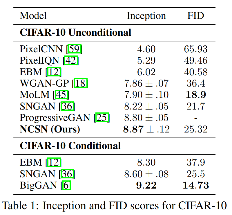
- state-of-the-art inception score of \(8.87\) on CIFAR-10
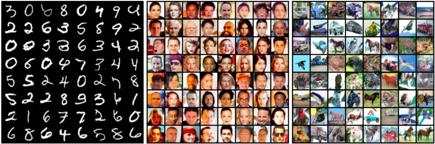
Figure 5: Random samples using annealed Langevin dynamics for a) MNIST b) CelebA c) CIFAR-10
Sampling Dynamics
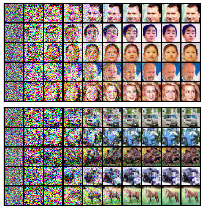
Figure 6: Intermediate samples of annealed Langevin dynamics.
Compared to other Methods
Conclusion
- New likelihood-free generative modeling framework
- Reach state-of-the-art inception score on CIFAR-10
- Not clear how well this methods scales to higher dimensions