Physics-guided Neural Networks (PGNN)
Anuj Karpatne*, William Watkins†, Jordan Read†, & Vipin Kumar*
*Department of Computer Science, University of Minnesota, †United States Geological Survey
Presented By
Andreas Munk
amunk@cs.ubc.ca
April 12, 2021
Table of Contents
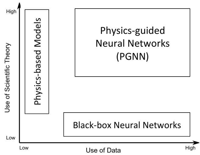
- Where is the physics in modern machine learning?
- Phisycs-guided Neural Networks (PGNN) cite:karpatne2017physics
- Constructing Hybrid-Physics-Data models
- Using physics-based loss functions
- Experiments
- Lake temperature modeling
- Physical inconsistency for lake temperature modeling
- Loss function for lake temperature modeling
- Results
- References
Where is the physics in modern machine learning?
- Neural networks (NN) are used for black-box modeling to solve regression and classification problems
- We cannot know if NNs even approximately captures underlying physical mechanics
- Even if they produce small test scores (e.g. mean-square-error (MSE))
- This obfuscates the functional relationship between input (\(x\)) and output
(\(y\)) variables
- Potentially impedes further scientific discoveries
- Arguably, this “issue” is less relevant when modeling a statistical
relationship between \(x\) and \(y\) - i.e. \(p_{\theta}(y|x)\).
Assume a “true” functional relationship between \(x\) and \(y\) with a noise term, \[y = f(x) + \epsilon\]
Any discrepancy between a learned function \(f_{\theta}\) and the true function \(f\) may be summarized as uncertainty associated with \(p_{\theta}(y|x)\)
- The perspective taken in this presentation is that we care about the functional relation between \(x\) and \(y\)
Phisycs-guided Neural Networks (PGNN) karpatne2017physics
- Combine neural networks with scientific knowledge of physics-based models
- Introduce an additional loss term that penalizes “flawed” relationships
between input and output variables under the neural network model
- The penalization is defined using known physical mechanics underlying the problem at hand
- These mechanics do not (necessarily) solve the problem, but encode certain relationship between (subsets) of the variables involved
- This framework can effectively be viewed as constraining the training of the neural networks
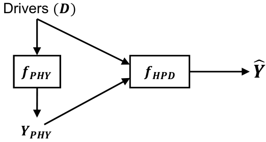
Constructing Hybrid-Physics-Data models
- Consider input variables (observable data or “drivers”) \(D\in\gD\) and target variable(s) \(Y\in\gY\)
- Standard neural network model
- \(f_{\mr{NN}}:\gD \rightarrow \gY\) with parameters \(\theta_{\mr{NN}}\)
- physics-based model
- \(f_{\mr{PHY}}:\gD \rightarrow \gY\)
- Hybrid model
- \(f_{\mr{HPD}}:\gX=\gD\times\gY \rightarrow \gY\) with parameters \(\theta_{\mr{HPD}}\)
- Also takes outputs from the physics based model
- Define \(\hat{Y}_{\mr{NN}}=f_{\mr{NN}}(D)\) and \(\hat{Y}_{\mr{HPD}}=f_{\mr{HPD}}(D,\hat{Y}_{\mr{NN}})\)
Using physics-based loss functions
Consider the following minimization problem
\[ \argmin_{\theta_{i}} \gL(\theta_{i})=\argmin_{\theta_{i}} \underbrace{\gL_{\mr{standard}}(\theta_{i})}_{\mr{"standard~loss"}} + \underbrace{\lambda R(\theta_{i})}_{\mr{regularization}} + \underbrace{\lambda_{\mr{PHY}}\gL_{\mr{PHY}}(\theta_{i})}_{\mr{Physical~Inconsistency}}, \quad i\in\tub{\mr{NN},\mr{HPD}}, \]
with \(\lambda\) and \(\lambda_{\mr{PHY}}\) being hyperparameters
- The Physical Inconsistency “measures constraint violations”
- Define equality and inequality constraints \[ \gG(Y,D) = 0 \quad \gH(Y, D) \leq 0 \]
- Both \(\gG\) and \(\gH\) are generic forms of physics-based (differentiable)
equations. Both forms captures a physics-based relationship between the
variable \(D\) and \(Y\).
- For instance let \(D\) describe time and Y the position of an object. If we know that the object moves with constant velocity (\(v\)) we can describe it’s position according to \(Y=f(D)=v\cdot D + Y_{0}\).
- Use the knowledge of the velocity to relate \(Y\) and \(D\), e.g. \(\gG(Y,D)=Y-(v\cdot D + Y_{0})\Rightarrow \gG(f(D),D)=0\)
- Leading to the following loss term (framed as soft constraints)
\[ \gL_{\mr{PHY}}(\theta_{i}) = \norm{\gG(f_{\mr{i}}(D),D)}^{2} + \mr{ReLU}(\gH(f_{\mr{i}}(D),D)) \quad i\in\tub{\mr{NN},\mr{HPD}} \]
Experiments
Lake temperature modeling
- Predict lake temperatures \(Y\) using PGNN
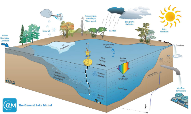
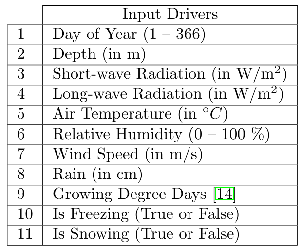
Figure 1: Input variables \(D\)
Physical inconsistency for lake temperature modeling
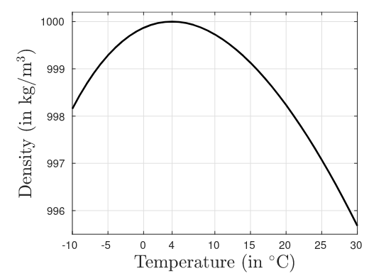
Temperature-density relationship of water
Denisty-depth relationship
- Density is monotonically increasing with depth
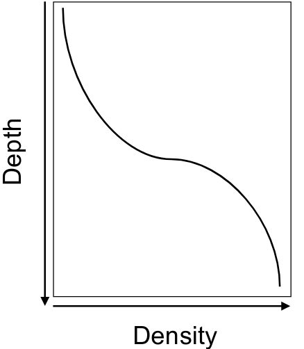
Figure 2: Sketch of depth and density relationship
Consider two depths \(d_{1}\) and \(d_{2}\) at time \(t\), then the density as a function of depth and time \(t\) must satisfy
\[ \rho(d_{1},t) - \rho(d_{2},t) \leq 0, \quad d_{1} \leq d_{2} \]
- We can use the above requirement to construct the inequality constraint \(\gH\)
- Consider the regular grid of \(n_{d}\) depth values and \(n_{t}\) time-steps
- Consider \(\hat{\rho}(d_{k},t)=\rho(f_{i}(D))\), where \(\rho(\cdot)\) is from \eqref{eq:rho}, the depth value and time value in \(D\) are equal \(d_{k}\) and \(t\) respectively, and \(f\) is a function, e.g. \(f_{\mr{PHY}}\)
- Define \(\Delta(k, t) = \hat{\rho}(d_{k}, t) - \hat{\rho}(d_{k+1}, t)\), with \(k\in\tub{1,\dots,n_{d}}\)
The physics regularized loss term then becomes
\[ \gL_{\mr{PHY}}(\theta_{i}) = \frac{1}{n_{t}(n_{d}-1)}\sum_{t=1}^{n_{t}}\sum_{k}^{n_{d}-1}\mr{ReLU}(\Delta(k,t)), \]
- Which we can differentiate with respect to \(\theta_{i}\)
Loss function for lake temperature modeling
- \(n\) is number of data points
- \(n_{d}\) is the number of unique depth measurements (different depth values)
- \(n_{t}\) is the number of unique time measurements (day of year)
- \(\Delta(k,t)\) is part of the physical inconsistency loss, as defined earlier
Results
Models and their notation
- NN, SVM, LSBoost: to a standard neural network model trained without physical knowledge, support vector machines, and least squared boosted regression tress
- PHY: A state-of-the-art general lake model (simulator)
- PGNN0: uses \(f_{\mr{PHY}}\) (i.e. takes simulated temperatures as additional arguments), but does not use \(\gL_{\mr{PHY}}\)
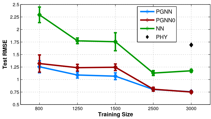
- PGNN: The proposed method
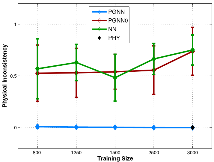
- Define the physical inconsistency metric - a number representing the fraction of times the density constraint is violated
Root mean squared error (RMSE) and physical inconsistency
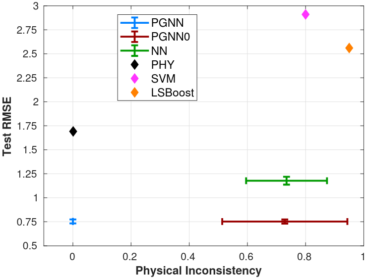
Figure 3: Lake Mille Lacs
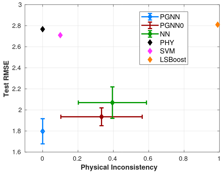
Figure 4: Lake Mendota
Relation to training size (Lake Mille Lacs)
Density-depth relationship
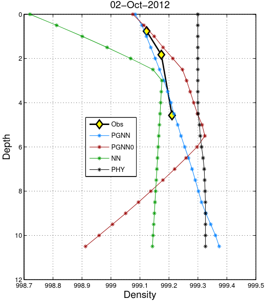
Figure 5: Lake Mille Lacs
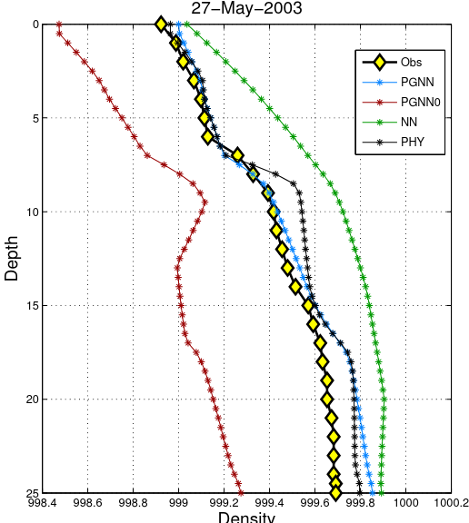
Figure 6: Lake Mendota